Inventory management is a crucial aspect of the automotive industry, as it directly impacts customer satisfaction, revenue, and profitability. 

Here you need more than just elbow grease – you need metrics. Why does it matter, you ask? To ensure efficient inventory management, it’s essential to track and measure key performance indicators (KPIs). 

They’re the real MVPs in ensuring everything,from the assembly line to the showroom floor, is firing on all cylinders.

Now, if you’re ready to dive deep into the world of automotive inventory management, you’re in for a treat. 

This blog is your go-to guide, decoding the 20 most crucial metrics that can make or break the game. 

Get ready to steer your way to success with the most crucial metrics in the automotive industry and get the formulas to track them!

1. Inventory Turnover Ratio

Inventory turnover is a critical metric that measures the number of times inventory is sold and replaced within a given period. It is the core of your supply chain, measuring how quickly your inventory is cycling through your business. 

A high turnover indicates agility and responsiveness, while a low one might signal sluggishness and potential issues.

Calculation of Inventory Turnover Ratio

The inventory turnover ratio is calculated by dividing COGS by average inventory on hand. The formula is:

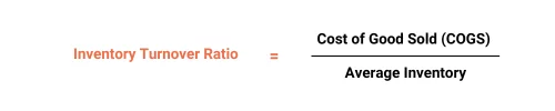
Break it down, and you’ll see it’s all about finding that sweet spot between what you’ve sold and what’s in your garage.

If your COGS for the year is $5 million, and your average inventory hovers around $2 million, your inventory turnover ratio would be 2.5 times. Easy peasy, right?

If your inventory turnover ratio is hitting the high notes, congratulations! You’re operating in the fast lane. It suggests that your inventory is zipping through the supply chain, minimizing holding costs, and maximizing cash flow. 

In the automotive world, this agility means staying ahead of market trends, meeting customer demands promptly, and optimizing your capital.

On the flip side, a low inventory turnover ratio might indicate that your wheels are spinning, but you’re not covering much ground. This could mean overstocking, slow-moving parts, or missed opportunities. 

So, ideally, you want to find the sweet spot. A turnover ratio that’s not too high to risk stock outs but not too low to choke your cash flow. This balance ensures that you’re riding the wave of demand without wiping out on excess inventory.

2. Stockout Rate 

So, what’s this stockout rate all about? Picture this: a customer walks into your dealership or browses your online store, eagerly searching for that elusive part. But, – it’s out of stock! That is a stockout, and the stockout rate is the frequency at which this happens. 

A high stockout rate can throw a wrench into your customer satisfaction and revenue streams.

Calculation of Stockout Rate

Stockout rate is calculated by dividing the number of stockouts by the total number of customer orders. The formula is:

For example, if you had 10 stock outs in a month, out of a total demand of 200 units, your stockout rate would be 5%. 

Stockouts aren’t just a bummer for customers; they’re a revenue pothole for your business. Every time a customer walks away empty-handed, that’s potential revenue lost. So keep those shelves stocked, and you’ll keep customers coming back for more.

Pro Tip: Use forecasting tools to predict future demand based on historical data, market trends, and external factors. Accurate demand forecasting helps in optimizing inventory levels and minimizing the risk of stockouts.

3. Fill Rate 

Fill rate measures the percentage of customer orders that are fulfilled from existing inventory. It’s an essential metric for ensuring that inventory levels are sufficient to meet customer demand. 

Now, why is fill rate the unsung hero in the automotive supply chain?

☑️ In an industry where precision matters, meeting customer orders promptly is non-negotiable. A high fill rate ensures that when your customers rev up their engines, they’re not left waiting for missing parts. It’s the key to keeping customer satisfaction on cruise control.

☑️ Consistently meeting customer orders builds trust – a commodity more valuable than gold in the automotive business. A high fill rate signals reliability, and in an industry where customers depend on your parts to keep their vehicles running, trust is your best insurance against competitors.

How to Calculate Fill Rate in the Automotive Industry:

Now, let’s pop the hood and take a look at how to calculate fill rate in the automotive industry.

The formula is straightforward: 

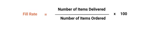
It’s about measuring the success of delivering complete orders.

For example, if a customer orders 10 items, and you deliver 9, your fill rate would be 90%. Simple math, but the impact on customer satisfaction and your bottom line is profound.

4. Stock Velocity

Stock Velocity, also known as Inventory Velocity, is a metric that measures the speed at which inventory is sold and replaced over a specific period. It reflects how efficiently a business is managing its inventory turnover and the rate at which products are moving through the supply chain.

The formula for calculating Stock Velocity involves two primary components:

High stock velocity indicates that inventory is moving swiftly, reducing the amount of capital tied up in unsold goods. This efficiency contributes to better working capital management.

Additionally, stock velocity metrics provide valuable insights for strategic decision-making. Businesses can use this data to optimize inventory levels, streamline ordering processes, and identify top-performing products.

5. Carrying Costs 

Carrying costs, also known as holding costs, refer to the expenses associated with holding and storing inventory. In the automotive industry, where precision is key, these costs extend beyond the physical storage space. 

They encompass everything from insurance and taxes to the opportunity cost of tying up capital in unsold inventory.

Calculation of Carrying Cost

Calculating carrying costs involves considering various factors associated with holding and storing inventory. The formula to calculate carrying costs is generally expressed as a percentage of the inventory value. Here’s the basic formula:

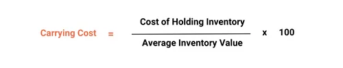
Now, let’s break down the components of this formula:

• Cost of Holding Inventory

This includes expenses related to holding and storing inventory, such as warehousing costs, insurance, security, utilities, and any additional expenses specific to your business.

• Average Inventory Value

Calculate the average inventory value by adding the beginning inventory value to the ending inventory value and dividing the result by 2. 

Average Inventory Value = (Beginning Inventory + Ending Inventory) / 2

The inventory value can be determined based on the cost of goods or the selling price, depending on your business model and industry practices.

• Percentage

Multiply the ratio of the Cost of Holding Inventory to the Average Inventory Value by 100 to express the carrying costs as a percentage.

Example: Let’s say you have the following figures for a certain period:

• Beginning Inventory: $100,000
• Ending Inventory: $120,000
• Cost of Holding Inventory: $15,000

Average Inventory Value = 100,000 + 120,000 / 2 = 110,000

Carrying Cost = (15,000 / 110,000) × 100 = 13.64%

So, in this example, the carrying cost is approximately 13.64% of the average inventory value.

It’s worth noting that the components and the way carrying costs are calculated can vary between businesses. Some may include additional factors like taxes, obsolescence costs, or opportunity costs of capital. Therefore, it’s essential to tailor the formula to match the specific needs and circumstances of your business.

To minimize carrying costs you can use strategies like optimizing inventory levels, streamlining supply chain processes, implementing just-in-time (JIT) inventory management, and using data analytics to forecast demand and optimize inventory levels.

6. Backorder Rate 

Tracking backorder rate is essential to ensure that inventory levels are sufficient to meet customer demand. 

Backorder rate measures the frequency at which inventory is depleted and cannot be replenished in time to meet customer demand. 

The relevance of backorders is twofold: it signals high demand for certain items, but it also poses challenges in meeting customer expectations promptly. 

Calculating Backorder Rate:

Backorder rate is calculated by dividing the number of backorders by the total number of customer orders. 

The formula is:

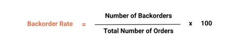
Breaking it down, you’re measuring the percentage of orders that couldn’t be fulfilled immediately due to items being out of stock. 

For example, if you had 20 backorders out of 100 total orders, your backorder rate would be 20%.

---

Expert Tip: How do you navigate the challenge of backorders to enhance the customer experience? Here are the expert tips:

• Accurate Demand Forecasting

Invest in robust demand forecasting tools. Understanding the ebb and flow of demand helps you anticipate which items are likely to face shortages, allowing you to mitigate backorders proactively.

•  Safety Stock and Inventory Buffer

Maintain a safety stock – a reserve of inventory beyond expected demand. This acts as a buffer, absorbing sudden spikes in demand and reducing the likelihood of backorders during peak periods.

• Real-Time Inventory Visibility

Implement systems that provide real-time visibility into your inventory. Knowing what’s in stock, what’s on order, and what’s en route allows you to make informed decisions and manage backorders effectively.

---

7. Order Cycle Time 

Order cycle time measures the time it takes to fulfill a customer order, from receipt to delivery. Tracking order cycle time is essential to ensure that orders are fulfilled promptly and efficiently. 

Efficient order cycle times translate directly into satisfied customers. When orders are processed swiftly, customers get what they need when they need it. This not only builds trust but also positions your brand as a reliable player in the competitive automotive landscape.

Moreover, short order cycle times enable your supply chain to respond rapidly to market changes and customer demands. Whether it’s a surge in orders or a change in product preferences, an agile supply chain ensures you stay ahead of the curve.

Measurement and Analysis of Order Cycle Time

Breaking it down, you’re calculating the average time it takes to process and fulfill an order. This includes the time from order placement to shipment and delivery.

Key Metrics to Analyze:

1. Processing Time: The time it takes to process an order internally.
2. Lead Time: The time it takes from order placement to the arrival of the product.
3. Delivery Time: The time it takes for the product to reach the customer after leaving your facility.

---

Expert Tip: Regularly analyze order cycle time to identify bottlenecks, inefficiencies, or areas for improvement. Use customer feedback, historical data, and performance metrics to refine and optimize the process continually.

---

8. Demand Forecast Accuracy 

Demand forecast accuracy measures the degree to which predicted demand matches actual demand. Tracking demand forecast accuracy is essential to ensure that inventory levels are optimized and customer demand is met. 

By predicting future demand, you can strategically optimize your inventory. This means maintaining optimal stock levels, preventing overstock or stockouts, and ultimately, maximizing efficiency and profitability.

Accurate forecasting is the key to delivering a seamless customer experience. When customers find what they need when they need it, it’s not just a sale – it’s a step towards building lasting loyalty and satisfaction.

Metrics for Evaluating Forecast Accuracy

Now, let’s pull over and inspect the metrics that gauge the accuracy of your forecasting efforts.

1. Mean Absolute Percentage Error (MAPE)

• MAPE measures the percentage difference between actual demand (Ai) and forecasted demand (Fi​) for each period, providing an average accuracy rate.

2. Mean Absolute Deviation (MAD)

MAD calculates the average absolute difference between actual and forecasted values, providing a measure of forecast accuracy in the original unit.

3. Tracking Signal

The tracking signal helps identify whether the forecast is biased or unbiased by examining the ratio of cumulative forecast error to MAD.

9. Lead Time Metrics 

Lead time measures the time it takes for inventory to arrive after it’s ordered. Tracking lead time metrics is essential to ensure that inventory levels are sufficient to meet customer demand.

It includes various activities, such as ordering, shipping, receiving, and inspection. 

Here are some important lead time metrics for inventory management in the automotive industry:

Lead Time Metrics	Definition	Formula
Supplier Lead Time (SLT)	Time for a supplier to deliver parts after receiving an order.	SLT= Processing Time+Manufacturing Time+Transportation Time
Total Lead Time (TLT)	Sum of Supplier Lead Time (SLT) and Internal Lead Time (ILT). Represents the duration from order to product receipt.	TLT= SLT+ILT
Internal Lead Time (ILT)	Time spent on internal processes after receiving parts from the supplier.	ILT=Receiving Time+Inspection Time+Storing Time
Lead Time Variability (LTV)	Measures inconsistency in lead times for a specific supplier or part.	LTV = (Average Lead Time / Standard Deviation of Lead Times) ​×100
Inventory Turns	Measures how often inventory is sold and replaced within a specific period.	Inventory Turns = Average Inventory / Cost of Goods Sold​
Days Inventory Outstanding (DIO)	Measures the average number of days to sell inventory.	DIO =Average Inventory / (Cost of Goods Sold Number of Days in Period)
GMROI (Gross Margin Return on Investment)	Measures the profitability of inventory management.	GMROI = Average Inventory Investment / Gross Margin​
Supply Chain Cycle Time	Measures the total time for designing, producing, and delivering a product. Includes lead times and transportation times.	Supply Chain Cycle Time = Lead Time + Production Time + Transportation Time

10. Stock-to-Sales Ratio

The Stock-to-Sales Ratio is a vital metric that quantifies the relationship between the amount of stock a business holds and its sales over a specific period. It serves as a dynamic indicator of how well a company is managing its inventory in alignment with consumer demand.

Purpose:

• Offers insights into inventory efficiency by gauging the balance between supply and demand.
• Guides strategic decision-making by indicating whether inventory levels are aligned with sales performance.
• Enables businesses to identify overstock or understock situations, optimizing resource allocation.

Calculating Stock-to-Sales Ratio

• Average Stock Level: Sum of the beginning and ending stock levels divided by 2.

• Net Sales: Total sales minus returns and allowances.

A high Stock-to-Sales Ratio suggests that inventory levels are proportionate to sales, indicating efficient management. Conversely, a low ratio may signify overstock, tying up capital and potentially leading to markdowns or obsolescence.

Moreover, a balanced Stock-to-Sales Ratio ensures that inventory matches consumer demand. This harmony prevents stockouts, boosting sales and customer satisfaction. On the flip side, an imbalance can result in missed sales opportunities or excess carrying costs.

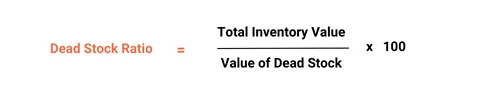
11. Dead Stock Ratio

Dead stock, also known as obsolete inventory, refers to products that haven’t sold within a defined period and are unlikely to sell in the future. Identifying dead stock involves scrutinizing sales data, historical demand patterns, and market trends.

The repercussions of dead stock extend beyond individual products, significantly influencing the holistic health of your inventory. Storing dead stock incurs unnecessary warehouse expenses, contributing to higher operational costs.

It’s calculated as follows:

12. ABC Analysis

ABC Analysis is a method of classifying items in an inventory based on their importance. It stems from the Pareto Principle, asserting that a small percentage of items contribute to the majority of the value or impact.

It focuses resources on items that have the most significant impact on overall efficiency, cost, and customer satisfaction.

Class	Percentage of Items	Contribution to Overall Value	Management Requirements
A-Class (High-Priority)	Approximately 20%	Significant contribution	Requires close monitoring, strategic planning, and efficient management due to their critical role in the supply chain.
B-Class (Medium-Priority)	Around 30%	Moderate impact	Requires regular attention but not as intensive management as A-Class items.
C-Class (Low-Priority)	About 50%	Minimal contribution	Generally requires standard inventory management practices with less frequent review.

13. Just-in-Time Metric

Just-in-Time (JIT) is an inventory management philosophy that emphasizes producing or receiving goods precisely when needed in the production process. It helps in minimizing excess inventory, and promoting efficiency throughout the supply chain.

Principles of JIT metrics:

• Demand-driven production
• Elimination of waste
• Continuous improvement

To gauge the success of JIT implementation, businesses utilize key metrics that provide insights into its efficiency:

• Lead Time Reduction: Measures the time taken from order placement to product delivery.

• Inventory Turnover: Evaluates how quickly inventory is sold and replaced within a specific period.

• Stockouts: Tracks instances where demand exceeds available inventory, indicating potential disruptions in the JIT flow.

• Supplier Reliability: Assesses the consistency and reliability of suppliers in delivering materials on time.

• Cycle Time: Measures the time it takes to complete one cycle of production, reflecting overall process efficiency.

14. On-Time Delivery (OTD)

OTD measures the percentage of deliveries that arrive on time, which is essential for maintaining operational efficiency. It is a critical performance indicator in supply chain management that assesses the reliability of suppliers and their ability to meet delivery deadlines. 

A high OTD percentage indicates that the supplier is reliable and can meet delivery deadlines, reducing the risk of production delays and ensuring timely delivery to customers.

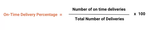
How to Calculate On-Time Delivery 

The formula is:

Here:

• Number of On-Time Deliveries: The count of deliveries that arrive according to the agreed-upon schedule.

• Total Number of Deliveries: The overall number of deliveries within the specified timeframe.

15. Supplier Risk Index

The supplier risk index evaluates the overall risk associated with a supplier, considering factors like geopolitical risks, financial stability, and quality control. 

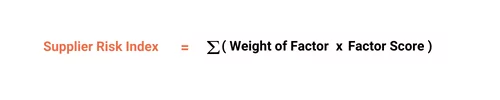
How to Calculate Supplier Risk Index

Calculating the Supplier Risk Index involves assigning weights to different risk factors based on their significance and aggregating them to derive an overall risk score. 

The formula may vary depending on the specific criteria and weights assigned by the organization. A simplified formula could be:

Here:

• Weight of Factor: The importance assigned to each risk factor in the overall assessment.
• Factor Score: The score assigned to the supplier for each specific risk factor.

A low supplier risk index indicates that the supplier is reliable, stable, and has a proven track record of delivering high-quality parts. 

This metric helps automotive manufacturers mitigate risks associated with supplier failure, ensuring a stable supply chain and minimizing the likelihood of production disruptions.

16. Economic Order Quantity (EOQ) 

Economic Order Quantity (EOQ) determines the optimal order quantity that minimizes total inventory costs. In the automotive industry, where precision and efficiency are paramount, understanding EOQ is crucial for maintaining a lean yet responsive inventory.

• EOQ minimizes the total costs associated with ordering and holding inventory.

• It balances the costs of ordering too frequently (ordering costs) with the costs of holding excess inventory (carrying costs).

It also helps maintain an optimal inventory level, preventing stock outs that could lead to production delays or excess inventory that incurs carrying costs.

Moreover, by optimizing order quantities, EOQ allows businesses to free up cash that would otherwise be tied up in excess inventory.

The EOQ formula provides the magic number for the ideal order quantity. The formula is as follows:

• D represents the demand for the product.
• S denotes the ordering cost per order.
• H signifies the holding cost per unit per year.

17. Shrinkage Rate 

Shrinkage in automotive inventory refers to the loss or reduction in inventory levels due to various factors, including theft, damage, errors, or other unforeseen circumstances.

Types of Shrinkage:

• Internal Shrinkage: Losses that occur within the organization, such as employee theft, errors in record-keeping, or mishandling of inventory.

• External Shrinkage: Losses caused by external factors like theft, damage during transportation, or issues within the supply chain.

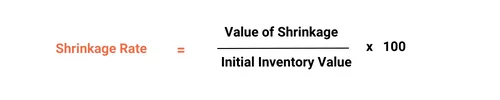
The formula for calculating the Shrinkage Rate is as follows:

Where:

• Value of Shrinkage is the monetary value of lost or damaged inventory.
• Initial Inventory Value is the total value of the initial inventory.

To effectively guard against shrinkage, businesses should implement a combination of physical security measures, employee training, and technology solutions. 

Technology solutions include advanced tracking systems, RFID technology, and inventory management software. Regular audits and inspections should also be conducted to identify and address discrepancies. 

18. Lead Time Accuracy

Lead Time Accuracy is a metric that evaluates how well the predicted or expected lead time aligns with the actual time it takes to receive goods or materials. In the context of supply chain and inventory management, lead time refers to the time elapsed between placing an order and receiving the ordered items.

How to Calculate Lead Time Accuracy: The calculation of Lead Time Accuracy involves comparing the predicted lead time with the actual lead time and expressing it as a percentage. 

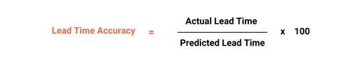
Here:

• Actual Lead Time: The real-time duration between order placement and the arrival of the ordered items.

• Predicted Lead Time: The anticipated or estimated time provided by suppliers or the internal forecasting system.

Accurate lead time predictions are crucial for effective supply chain planning. They enable businesses to align their production and inventory schedules with the expected arrival of goods.

Additionally, meeting or exceeding predicted lead times contributes to customer satisfaction. It ensures that products are available when expected, enhancing the overall customer experience.

19. Delivery Deviation Rate

Delivery Deviation Rate is a crucial metric in supply chain management that assesses the extent to which actual deliveries deviate from the initially agreed-upon schedule or expected timeframes. 

This metric provides insights into the reliability of suppliers and the consistency of delivery timelines.

Consistent delivery timelines contribute to customer satisfaction. Deviations can impact customer expectations and overall experience.

Deviations in delivery schedules can lead to disruptions in inventory management. Businesses may face challenges with overstock or stockout situations.

Moreover, high Delivery Deviation Rates may indicate potential risks in the supply chain, allowing businesses to identify and address issues promptly.

How to Calculate Delivery Deviation Rate

The calculation of Delivery Deviation Rate involves comparing the actual delivery dates with the scheduled or expected delivery dates and expressing it as a percentage. The formula is as follows:

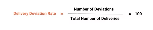
• Number of Deviations: The count of deliveries that deviate from the initially agreed-upon schedule.

• Total Number of Deliveries: The overall number of deliveries within the specified timeframe.

---

Expert Tip: 

For managing and improving delivery deviation rate implement real-time tracking systems to monitor the progress of deliveries and detect any deviations as they occur. 

Also, collaborate closely with suppliers on joint planning and forecasting to align expectations and reduce the likelihood of deviations.

Moreover, use technology solutions, such as advanced supply chain management software, to automate and optimize delivery scheduling, reducing the chances of deviations.

---

20. Customer Satisfaction Scores (CSAT)

CSAT, or Customer Satisfaction Score, is a metric used to measure how satisfied customers are with a specific interaction, product, or service. In the context of the automotive industry, CSAT gauges the satisfaction levels of customers post-purchase, providing valuable insights into their overall experience.

How to Calculate CSAT

Calculating CSAT involves collecting feedback through surveys. Here’s the typical process:

• Survey Question: Customers are asked a direct question related to satisfaction, often phrased as, “How would you rate your satisfaction with [product/service/interaction]?”

• Rating Scale: Respondents provide their feedback using a numerical scale, commonly ranging from 1 to 5 or including options like “Very Satisfied,” “Satisfied,” “Neutral,” “Dissatisfied,” and “Very Dissatisfied.”

• Calculation: The CSAT score is then calculated by finding the percentage of positive responses (e.g., the number of “Satisfied” or “Very Satisfied” responses) out of the total number of responses.

In a competitive market, a high CSAT score can be a significant differentiator. It gives an edge over competitors and positions the brand as one that prioritizes customer satisfaction. 

Understanding and addressing customer satisfaction issues can help in retaining existing customers. It is often more cost-effective to retain satisfied customers than to acquire new ones.

Turn Data Into Results With Dealership Analytics from Autosoft

To wrap up, effective inventory management is crucial for the success of any automotive business. By adopting a holistic approach that considers all aspects of inventory management, automotive companies can optimize their operations and drive growth. 

Now, are you tired of sifting through endless data without seeing any tangible results? Autosoft provides actionable insights that help you understand your dealership’s needs and apply changes that drive real results.

Receive alerts when action is required in your sales or service departments, so you can stay on top of your game and address any issues promptly. Leverage color-coded visuals that make it easy to quickly make decisions based on historical data, ensuring that you’re always working with the most up-to-date information.

Moreover, Autosoft tracks real-time market data, enabling you to make profitable inventory decisions. Don’t let data overwhelm you – turn it into results with Autosoft’s Dealership Analytics. Schedule your demo today!